from __future__ import annotations

import matplotlib.pyplot as plt
import numpy as np

from multinterp.rectilinear._multi import MultivaluedInterp

def squared_coords(x, y):
    return x**2 + y**2


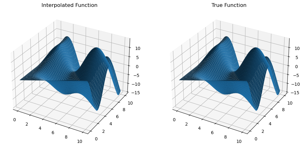
def trig_func(x, y):
    return y * np.sin(x) + x * np.cos(y)

x_grid = np.geomspace(1, 11, 1000) - 1
y_grid = np.geomspace(1, 11, 1000) - 1
x_mat, y_mat = np.meshgrid(x_grid, y_grid, indexing="ij")

z_mat = np.asarray([squared_coords(x_mat, y_mat), trig_func(x_mat, y_mat)])

x_new, y_new = np.meshgrid(
    np.linspace(0, 10, 1000),
    np.linspace(0, 10, 1000),
    indexing="ij",
)

mult_interp = MultivaluedInterp(z_mat, [x_grid, y_grid], backend="cupy")
z_mult_interp = mult_interp(x_new, y_new).get()
z_true = np.asarray([squared_coords(x_new, y_new), trig_func(x_new, y_new)])

# Create a figure with two subplots
fig = plt.figure(figsize=(12, 6))

# Plot the interpolated function
ax1 = fig.add_subplot(1, 2, 1, projection="3d")
ax1.plot_surface(x_new, y_new, z_mult_interp[0])
ax1.set_title("Interpolated Function")

# Plot the true function
ax2 = fig.add_subplot(1, 2, 2, projection="3d")
ax2.plot_surface(x_new, y_new, z_true[0])
ax2.set_title("True Function")

plt.show()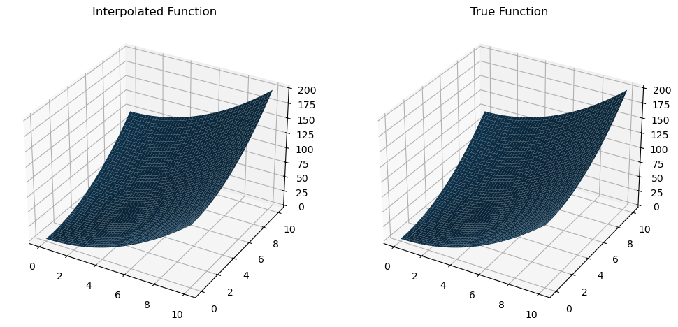

# Create a figure with two subplots
fig = plt.figure(figsize=(12, 6))

# Plot the interpolated function
ax1 = fig.add_subplot(1, 2, 1, projection="3d")
ax1.plot_surface(x_new, y_new, z_mult_interp[1])
ax1.set_title("Interpolated Function")

# Plot the true function
ax2 = fig.add_subplot(1, 2, 2, projection="3d")
ax2.plot_surface(x_new, y_new, z_true[1])
ax2.set_title("True Function")

plt.show()