Unstructured Interpolation using scipy - Multivariate Interpolation

This notebook uses examples from scipy documentation to demonstrate HARK’s UnstructuredInterp class.

from __future__ import annotations

import matplotlib.pyplot as plt
import numpy as np

from multinterp.unstructured import UnstructuredInterp

Suppose we have a collection of values for an unknown function along with their respective coordinate points. For illustration, assume the values come from the following function:

def function_1(x, y):
    return x * (1 - x) * np.cos(4 * np.pi * x) * np.sin(4 * np.pi * y**2) ** 2

The points are randomly scattered in the unit square and therefore have no regular structure.

rng = np.random.default_rng(0)
rand_x, rand_y = rng.random((2, 1000))
values = function_1(rand_x, rand_y)

Now suppose we would like to interpolate this function on a rectilinear grid, which is known as “regridding”.

grid_x, grid_y = np.meshgrid(
    np.linspace(0, 1, 100), np.linspace(0, 1, 100), indexing="ij"
)

To do this, we use HARK’s UnstructuredInterp class. The class takes the following arguments:

values: an ND-array of values for the function at the points
grids: a list of ND-arrays of coordinates for the points
method: the interpolation method to use, with options “nearest”, “linear”, “cubic” (for 2D only), and “rbf”. The default is 'linear'.

nearest_interp = UnstructuredInterp(values, (rand_x, rand_y), method="nearest")
linear_interp = UnstructuredInterp(values, (rand_x, rand_y), method="linear")
cubic_interp = UnstructuredInterp(values, (rand_x, rand_y), method="cubic")
rbf_interp = UnstructuredInterp(values, (rand_x, rand_y), method="rbf")

Once we create the interpolator objects, we can use them using the __call__ method which takes as many arguments as there are dimensions.

nearest_grid = nearest_interp(grid_x, grid_y)
linear_grid = linear_interp(grid_x, grid_y)
cubic_grid = cubic_interp(grid_x, grid_y)
rbf_grid = rbf_interp(grid_x, grid_y)

Now we can compare the results of the interpolation with the original function. Below we plot the original function and the sample points that are known.

plt.imshow(function_1(grid_x, grid_y).T, extent=(0, 1, 0, 1), origin="lower")
plt.plot(rand_x, rand_y, "ok", ms=2, label="input points")
plt.title("Original")
plt.legend(loc="lower right")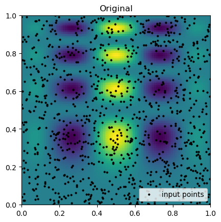

Then, we can look at the result for each method of interpolation and compare it to the original function.

fig, axs = plt.subplots(2, 2, figsize=(6, 6))
titles = ["Nearest", "Linear", "Cubic", "Radial basis function"]
grids = [nearest_grid, linear_grid, cubic_grid, rbf_grid]

for ax, title, grid in zip(axs.flat, titles, grids):
    im = ax.imshow(grid.T, extent=(0, 1, 0, 1), origin="lower")
    ax.set_title(title)

plt.tight_layout()
plt.show()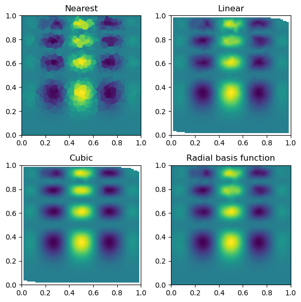

Another Example¶

def function_2(x, y):
    return np.hypot(x, y)

rng = np.random.default_rng(0)
rand_x = rng.random(20) - 0.5
rand_y = rng.random(20) - 0.5
values = function_2(rand_x, rand_y)
grid_x = np.linspace(min(rand_x), max(rand_x))
grid_y = np.linspace(min(rand_y), max(rand_y))
grid_x, grid_y = np.meshgrid(grid_x, grid_y)

nearest_interp = UnstructuredInterp(values, (rand_x, rand_y), method="nearest")
linear_interp = UnstructuredInterp(values, (rand_x, rand_y), method="linear")
cubic_interp = UnstructuredInterp(values, (rand_x, rand_y), method="cubic")
rbf_interp = UnstructuredInterp(values, (rand_x, rand_y), method="rbf")

nearest_grid = nearest_interp(grid_x, grid_y)
linear_grid = linear_interp(grid_x, grid_y)
cubic_grid = cubic_interp(grid_x, grid_y)
rbf_grid = rbf_interp(grid_x, grid_y)

plt.imshow(function_2(grid_x, grid_y).T, extent=(-0.5, 0.5, -0.5, 0.5), origin="lower")
plt.plot(rand_x, rand_y, "ok", label="input points")
plt.title("Original")
plt.legend(loc="lower right")

fig, axs = plt.subplots(2, 2, figsize=(7, 6))
titles = ["Nearest", "Linear", "Cubic", "Radial basis function"]
grids = [nearest_grid, linear_grid, cubic_grid, rbf_grid]

for _i, (ax, title, grid) in enumerate(zip(axs.flat, titles, grids)):
    im = ax.pcolormesh(grid_x, grid_y, grid, shading="auto")
    pts = ax.plot(rand_x, rand_y, "ok", label="input points")
    ax.set_title(title)

fig.legend(handles=pts, loc="lower center")
cbar = fig.colorbar(im, ax=axs)
for ax in axs.flat:
    ax.axis("equal")

plt.show()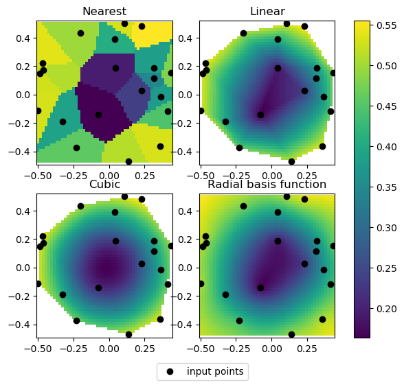

Unstructured Interpolators with Curvilinear Grids¶

def function_3(u, v):
    return u * np.cos(u * v) + v * np.sin(u * v)

rng = np.random.default_rng(0)
warp_factor = 0.1
x_list = np.linspace(0, 3, 10)
y_list = np.linspace(0, 3, 10)
x_temp, y_temp = np.meshgrid(x_list, y_list, indexing="ij")
rand_x = x_temp + warp_factor * (rng.random((x_list.size, y_list.size)) - 0.5)
rand_y = y_temp + warp_factor * (rng.random((x_list.size, y_list.size)) - 0.5)
values = function_3(rand_x, rand_y)

grid_x, grid_y = np.meshgrid(
    np.linspace(0, 3, 100), np.linspace(0, 3, 100), indexing="ij"
)

methods = ["nearest", "linear", "cubic", "rbf"]
nearest_interp, linear_interp, cubic_interp, rbf_interp = (
    UnstructuredInterp(values, (rand_x, rand_y), method=method) for method in methods
)

interp_funcs = [nearest_interp, linear_interp, cubic_interp, rbf_interp]
nearest_grid, linear_grid, cubic_grid, rbf_grid = (
    interp_func(grid_x, grid_y) for interp_func in interp_funcs
)

plt.imshow(function_3(grid_x, grid_y).T, extent=(0, 3, 0, 3), origin="lower")
plt.plot(rand_x.flat, rand_y.flat, "ok", ms=2, label="input points")
plt.title("Original")
plt.legend(loc="lower right")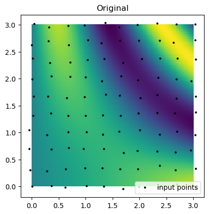

fig, axs = plt.subplots(2, 2, figsize=(6, 6))
titles = ["Nearest", "Linear", "Cubic", "Radial basis function"]
grids = [nearest_grid, linear_grid, cubic_grid, rbf_grid]

for ax, title, grid in zip(axs.flat, titles, grids):
    im = ax.imshow(grid.T, extent=(0, 3, 0, 3), origin="lower")
    ax.set_title(title)

plt.tight_layout()
plt.show()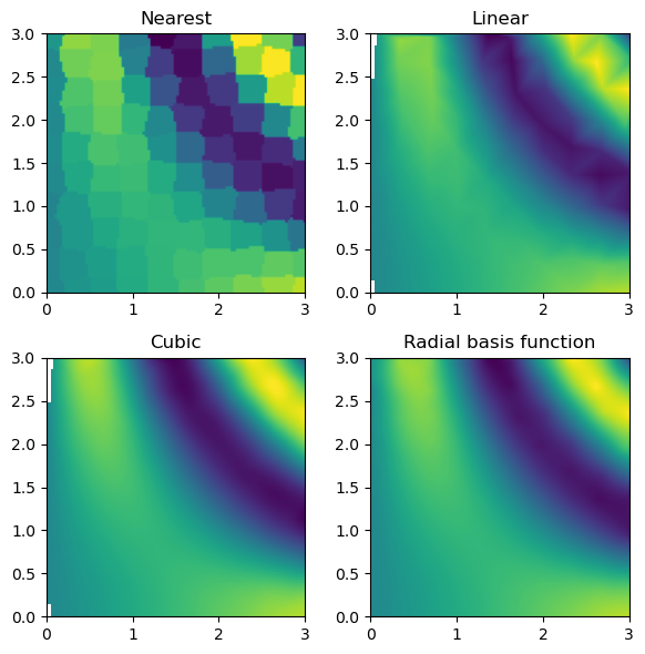

def function_4(x, y):
    return 3.0 * x**2.0 + x * y + 4.0 * y**2.0

rng = np.random.default_rng(0)
warp_factor = 0.2
x_list = np.linspace(0, 5, 20)
y_list = np.linspace(0, 5, 20)
x_temp, y_temp = np.meshgrid(x_list, y_list, indexing="ij")
rand_x = x_temp + warp_factor * (rng.random((x_list.size, y_list.size)) - 0.5)
rand_y = y_temp + warp_factor * (rng.random((x_list.size, y_list.size)) - 0.5)
values = function_4(rand_x, rand_y)

grid_x, grid_y = np.meshgrid(
    np.linspace(0, 5, 100), np.linspace(0, 5, 100), indexing="ij"
)

methods = ["nearest", "linear", "cubic", "rbf"]
nearest_interp, linear_interp, cubic_interp, rbf_interp = (
    UnstructuredInterp(values, (rand_x, rand_y), method=method) for method in methods
)

interp_funcs = [nearest_interp, linear_interp, cubic_interp, rbf_interp]
nearest_grid, linear_grid, cubic_grid, rbf_grid = (
    interp_func(grid_x, grid_y) for interp_func in interp_funcs
)

plt.imshow(function_4(grid_x, grid_y).T, extent=(0, 5, 0, 5), origin="lower")
plt.plot(rand_x.flat, rand_y.flat, "ok", ms=2, label="input points")
plt.title("Original")
plt.legend(loc="lower right")

fig, axs = plt.subplots(2, 2, figsize=(6, 6))
titles = ["Nearest", "Linear", "Cubic", "Radial basis function"]
grids = [nearest_grid, linear_grid, cubic_grid, rbf_grid]

for ax, title, grid in zip(axs.flat, titles, grids):
    im = ax.imshow(grid.T, extent=(0, 5, 0, 5), origin="lower")
    ax.set_title(title)

plt.tight_layout()
plt.show()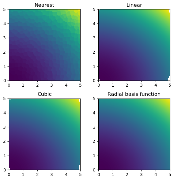

More complex functions¶

def function_5(*args):
    return np.maximum(
        0.0,
        1.0
        - np.exp(0.5 - np.prod(np.asarray(args) + 0.2, axis=0) ** (1.0 / len(args))),
    )

rng = np.random.default_rng(0)
rand_x, rand_y = rng.random((2, 1000))
values = function_5(rand_x, rand_y)

grid_x, grid_y = np.meshgrid(
    np.linspace(0, 1, 100), np.linspace(0, 1, 100), indexing="ij"
)

nearest_interp = UnstructuredInterp(values, (rand_x, rand_y), method="nearest")
linear_interp = UnstructuredInterp(values, (rand_x, rand_y), method="linear")
cubic_interp = UnstructuredInterp(values, (rand_x, rand_y), method="cubic")
rbf_interp = UnstructuredInterp(values, (rand_x, rand_y), method="rbf")

nearest_grid = nearest_interp(grid_x, grid_y)
linear_grid = linear_interp(grid_x, grid_y)
cubic_grid = cubic_interp(grid_x, grid_y)
rbf_grid = rbf_interp(grid_x, grid_y)

ax = plt.axes(projection="3d")
ax.plot_surface(
    grid_x,
    grid_y,
    function_5(grid_x, grid_y),
    rstride=1,
    cstride=1,
    cmap="viridis",
    edgecolor="none",
)
ax.scatter(rand_x, rand_y, values, c=values, cmap="viridis", label="input points")
plt.title("Original")
plt.legend(loc="lower right")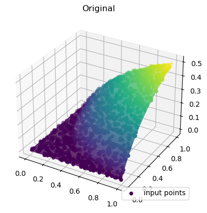

fig, axs = plt.subplots(2, 2, figsize=(6, 6), subplot_kw={"projection": "3d"})
titles = ["Nearest", "Linear", "Cubic", "Radial basis function"]
grids = [nearest_grid, linear_grid, cubic_grid, rbf_grid]

for ax, title, grid in zip(axs.flat, titles, grids):
    im = ax.plot_surface(
        grid_x, grid_y, grid, rstride=1, cstride=1, cmap="viridis", edgecolor="none"
    )
    ax.set_title(title)

plt.tight_layout()
plt.show()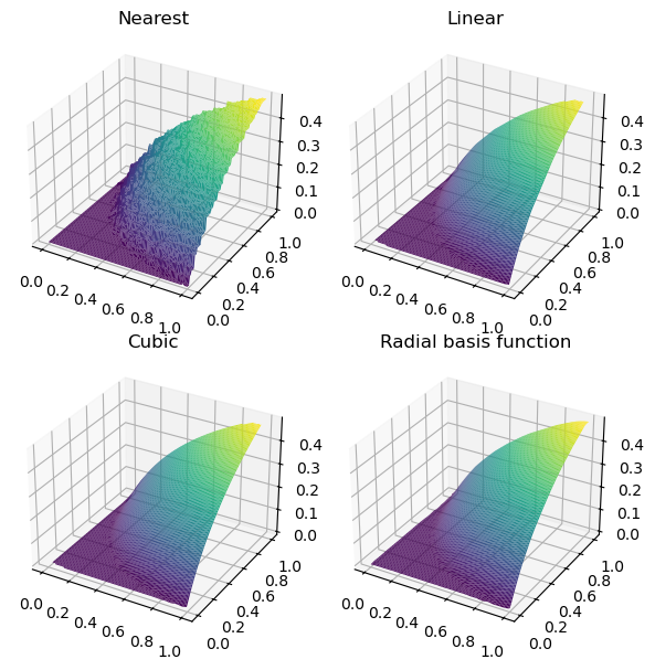

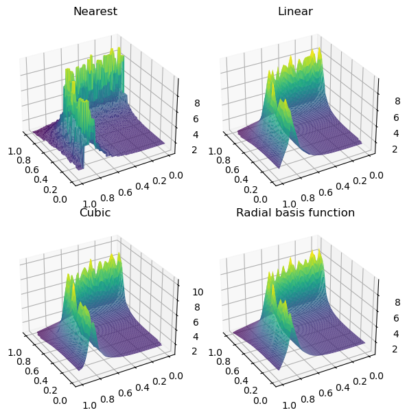
def function_6(x, y):
    return 1 / (np.abs(0.5 - x**4 - y**4) + 0.1)

rng = np.random.default_rng(0)
rand_x, rand_y = rng.random((2, 1000))
values = function_6(rand_x, rand_y)

grid_x, grid_y = np.meshgrid(
    np.linspace(0, 1, 100), np.linspace(0, 1, 100), indexing="ij"
)

nearest_interp = UnstructuredInterp(values, (rand_x, rand_y), method="nearest")
linear_interp = UnstructuredInterp(values, (rand_x, rand_y), method="linear")
cubic_interp = UnstructuredInterp(values, (rand_x, rand_y), method="cubic")
rbf_interp = UnstructuredInterp(values, (rand_x, rand_y), method="rbf")

nearest_grid = nearest_interp(grid_x, grid_y)
linear_grid = linear_interp(grid_x, grid_y)
cubic_grid = cubic_interp(grid_x, grid_y)
rbf_grid = rbf_interp(grid_x, grid_y)

ax = plt.axes(projection="3d")
ax.plot_surface(
    grid_x,
    grid_y,
    function_6(grid_x, grid_y),
    rstride=1,
    cstride=1,
    cmap="viridis",
    edgecolor="none",
)
ax.scatter(rand_x, rand_y, values, c=values, cmap="viridis", label="input points")
ax.view_init(30, 150)
plt.title("Original")
plt.legend(loc="lower right")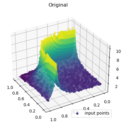

fig, axs = plt.subplots(2, 2, figsize=(6, 6), subplot_kw={"projection": "3d"})
titles = ["Nearest", "Linear", "Cubic", "Radial basis function"]
grids = [nearest_grid, linear_grid, cubic_grid, rbf_grid]

for ax, title, grid in zip(axs.flat, titles, grids):
    im = ax.plot_surface(
        grid_x, grid_y, grid, rstride=1, cstride=1, cmap="viridis", edgecolor="none"
    )
    ax.set_title(title)
    ax.view_init(30, 150)


plt.tight_layout()
plt.show()

Curvilinear

Piecewise Affine Interpolation

Unstructured

Regression Interpolation using scikit-learn